Image Compression with SVD and K-Means

Hello, this blog post serves a supplement to our course material in CS514. In class, we talked about and experimented with using Singular Value Decomposition as a form of image compression. Image compression can also be performed using another algorithm that we discussed in class, k-means. Unlike some of the other blog posts, this blog post will be somewhat experimental. I will be showing a comparison of the quality and compression ratio for SVD and k-means on this image of a mandrill from the SIPI image database.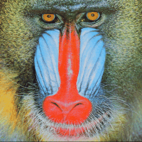

Simple SVD Compression

First I’ll start with a simple SVD compression like we covered in class. Below I show the approximations of the original image using the first 1, 5, 10, 25, 50, and 100 singular values.

As we already knew, taking a k-rank approximation of an image gives a reasonable good approximation of that image, especially when k is closer to the rank of the original image (in this case 200). To calculate our compression ratio, we assume that one color channel of an uncompressed image takes 200 x 200 = 40000 bytes for our 200 x 200 image while the k rank SVD takes 2 x (200 x k) x 2 bytes for our two N x k matrices of 16 bit floats (the singular values can be multiplied with U and then discarded). This means that we can calculate our compression ratio as 40000 / (4 x (200 x k))=50/k.

Using this formula, we can see that our solution does not work very well. The compression ratio at k=50 is 1, meaning that the “compressed” image is actually the same size as our original. At k=100, the ratio is 0.5, our compression has doubled the image size! At k = 25, the compression ratio is a decent 2, but we cannot get much better quality while still reducing the image size. One solution to this problem, which we will be trying in the next section, is to use a different approach for image compression.

K-Means Compression

We can use K-means to reduce the dimensionality of images by clustering the individual pixel values then mapping each pixel to its cluster centroid. This means that, if we have k clusters, we only need log(k) bits for each pixel and 3 * k bytes for each of the cluster centers. Below, I show the 2, 5, 10, 25, and 50 cluster approximations of our mandrill.

We can calculate our compression ratio this time using the formula 120000 / (40000 x ceil(log(k))/8 + 3 * k). This time the compression ratio 4.785643070787637 for 25 cluster and 3.9800995024875623 for 50. Thus, for this image, k-means is able to substantially reduce the file size while maintaining a reasonable image quality, unlike SVD.

SVD Compression on Chunks of The Image

However, we do not have to give up on SVD completely. SVD image compression can be improved by breaking the image up into smaller blocks of size b x b and calculating an SVD for each of these b x b matrices. For example, below I will show SVD with 1, 2, 3, 4, and 5 singular values on each 25x25 chunk of the image.

As you can see, this method performs much better for smaller rank approximations. Of course, smaller rank approximations also require more memory than simple SVD. We can calculate the compression ratio by dividing the memory used to store one block of the original image by the memory used to store one block of the compressed image. This equation is b^2 / (2 x (b x k) x 2) = b/(4k) as we need 2 x (b x k) x 2 bytes of memory to store the two b by k matrices of singular vectors (each entry in these matrices is a 2 byte floating point).

Using this equation, we can see that the compression ratio for the 3, 4, and 5 rank approximations of the 25 by 25 pixel chunks are 2.0833, 1.5625, and 1.25 respectively. We are still underperformed K-Means (and in fact our gains from simple SVD compression are fairly small), but this does show that SVD can be customized to the specific image. One advantage to this form of SVD is that it is very fast as the operations are performed over small matrices while K-Means is quite slow. This image may be too small to show the advantages of this form of SVD, and an advantage of this method that we do not utilize is the ability to use different ranks for different chunks.

More Complex Image

Next we will look at the following image.

As you can see, this image is larger and has a lot more color than our baboon. The first thing that is apparent to me in the comparison of compression algorithms is that the time to compress the image becomes much more relevant. The complex SVD and SVD are still very fast while K-means is prohibitively slow. Below I will show the 100 rank simple SVD, the rank 4 for approximation of 20 x 20 blocks, and 100-means compressed images.

The two SVD methods have the same compression ratios, but the complex SVD was closer to the original image. The Frobenius norm of the difference between the original image and the complex SVD image is 5135.225, compared to 5381.834. Therefore, the difference in these two methods is small, but the customizability allows the more complex one to perform better. The K-means has a much better compression ration and a much worse image, but the running time makes comparison for more clusters difficult.

Conclusions

In my experimentation, I had much better results with K-means than SVD. However, we also saw that SVD can be modified to improve performance and is a faster algorithm. There is no reason that would could not use different rank approximations for different chunks in our SVD algorithm to improve performance further.

We could also modify our K-Means algorithm to operate on chunks of the image as we did with SVD; this possibility deserves further inquiry in a future post that I may or may not make.

Final conclusions are that with these simple algorithms, K-means wins in Quality:Size ratio while SVD win in performance. Complex SVD does not do much better than regular SVD, but it is an improvement and further improvements could be made.

Link to Code

All the code that I used to generate the mandrill can be found on my github here. These files were designed to be easily customizable so that you could experiment for yourself.